Ports
At the start of a simulation, electric or magnetic fields are introduced into the simulation domain, applying an initial energy and signal input to the system. Some excitations only last one timestep, while most excitations are gradually applied over many timesteps. For the purpose of circuit designs, voltages and currents are also calculated to measure time-domain waveforms.
Internally, it’s implemented using excitation sources to set numerical values of the field at specified Yee cells. Weighting functions are used to further control the field’s pattern and polarization. Voltage and current are measured by probes, which integrate the electric and magnetic fields along 1D lines. Finally, lumped resistances often are needed to present specific impedances at locations where voltages and currents are measured.
Controlling these low-level entities for every simulation is inconvenient for the purpose of circuit designs. Hence, openEMS implements a high-level concept called ports, which creates appropriate entities automatically for common port types. This allows users to treat ports as the virtual 3D counterpart of physical ports on RF/microwave components, such as the standard 50 Ω input or output ports on circuit boards, signal generators, oscilloscopes, and especially Vector Network Analyzers (VNA).
Note
Ports are the most-commonly used form of excitations, this page presents a port-based view. For a description of non-port excitations (including Radar Cross Section), see Excitation Sources.
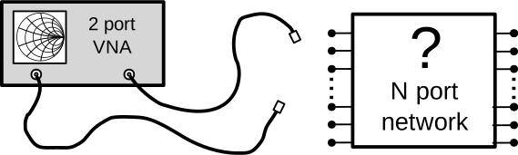
The “port” in openEMS serves a purpose similar to the physical
ports on Vector Network Analyzers and circuit boards. Both kinds of
ports are used to inject an input signal at a particular point in the
Device-Under-Test (DUT), and to measure what comes out at another point.
The DUT is thus characterized as a black box, solely represented using
its input-output relationships without an internal structure.
Note that port implementations are fundamentally different in
physical instruments (via circuits) and in openEMS simulations
(by loading numerical values into Yee cells). Image by Julien Hillairet,
from the scikit-rf project, licensed under BSD-3, modified for clarity.
Types
One can classify ports into two types, lumped ports and distributed ports.
API Reference
Port Type |
Matlab/Octave |
Python |
|---|---|---|
Lumped |
||
Curved |
||
Microstrip |
||
Stripline |
||
Coplanar Waveguide |
||
Coaxial |
||
Generic Waveguide |
||
Rectangular Waveguide |
||
Circular Waveguide |
Lumped Ports
A lumped port is the simplest and basic port type. It can be understood as a source that injects electromagnetic energy into the simulation at a defined position, providing an initial stimulus for the system. Simultaneously, a lumped resistor and a probe are also created at the same location as the port, allowing it to provide a matched load for the signal, and to measure the voltage or current at this region.
Lumped ports play a role similar to signal generators in circuit simulators. Both kinds of sources act like a voltage source or load with a resistive impedance, which are used to inject a signal to the Device-Under-Test or measure the DUT’s response, either from its own signal or from another port.
Limitation of the Lumped Port
A lumped port uses a constant-value electric field as the excitation signal, its physical size must be much smaller than the simulated structure to ensure the validity of the lumped-circuit approximation. If a significant distance exists between the end-points of a lumped port, simulation artifacts may occur.
A lumped port is a small 2D surface or 3D cube filled by an electric field, it can only be used to excite a two-conductor TEM transmission line, it cannot be used to excite hollow waveguides, and will perform poorly if the transmission lines requires an excitation field with a specific shape, polarization or contains multiple conductors, such as striplines, coplanar waveguides, differential pairs, or coaxial cables.
To avoid signal reflections, the lumped port must also have a lumped resistance matched to the characteristic impedance of the transmission line, which is problematic if the characteristic impedance of the transmission line is unknown.
Transmission Line Ports
Transmission line ports are designed for structures where the field distribution of the propagating mode is known: microstrip lines (MSL), striplines, coplanar waveguides (CPW), coaxial cables, and hollow metallic waveguides.
The key distinction from a lumped port is how the characteristic impedance and wave quantities are determined. A lumped port uses a user-specified Z₀ and a uniform electric field. Transmission line ports instead measure voltage and current at multiple positions along the line to directly separate the forward-traveling (incident) and backward-traveling (reflected) waves. The characteristic impedance is then extracted from the ratio of these wave quantities — consistent with the actual fields in the simulation, rather than depending on a user-provided value.
As a result, transmission line ports do not require a matched lumped termination resistance at the port plane. However, the far end of the transmission line still needs a proper termination, typically an absorbing boundary condition (PML or MUR) placed close to the line’s end, or a separate lumped resistance element.
Planar ports (MSL, Stripline, CPW, Coaxial)
These ports create the excitation at the port plane and place probes at multiple positions along the propagation direction. From the recorded voltages and currents the incident and reflected voltage waves are computed and S-parameters are derived, referenced to the extracted Z₀.
For a coaxial port, the excitation uses a radial electric field profile matching the TEM mode of the coaxial geometry.
Waveguide ports
Hollow metallic waveguides support only TE and TM propagation modes, not TEM. A lumped port cannot excite these correctly: it would see the waveguide as a DC short circuit and fail to launch energy above the cutoff frequency.
Waveguide ports in openEMS excite the desired mode (typically TE₁₀ for a rectangular waveguide) by applying a spatially-varying electric field profile matching the mode’s field distribution. The wave impedance is calculated analytically from the waveguide dimensions and the operating frequency. S-parameters are normalized to this wave impedance.
Feature Reference
Port Type |
Field Profile |
How many? |
Impedance Extraction |
|---|---|---|---|
Lumped |
Constant |
1 |
No |
Curved |
Constant |
1 |
No |
Microstrip |
Constant |
1 |
Yes |
Stripline |
Constant |
2 |
Yes |
Coplanar Waveguide |
Constant |
2 |
Yes |
Coaxial |
Radial |
1 |
Yes |
Generic Waveguide |
Manual Weighting Function |
1 |
No - Formula Only |
Rectangular Waveguide |
TE/TM Mode |
1 |
No - Formula Only |
Circular Waveguide |
TE/TM Mode |
1 |
No - Formula Only |
Usage
The following example adds two lumped ports to the simulation.
z0 = 50;

start = [-100 0 0];
stop  = [-100 0 50];
[CSX port{1}] = AddLumpedPort(CSX, 5, 1, z0, start, stop, [0 0 1], true);

start = [100 0 0];
stop  = [100 0 50];
[CSX port{2}] = AddLumpedPort(CSX, 5, 2, z0, start, stop, [0 0 1], false);
z0 = 50

port = [None, None]

start = [-100 0 0]
stop  = [-100 0 50]
port[0] = fdtd.AddLumpedPort(1, z0, start, stop, 'z', excite=1)

start = [-100 0 0]
stop  = [-100 0 50]
port[1] = fdtd.AddLumpedPort(2, z0, start, stop, 'z', excite=0)
See also
This page is incomplete. See the Legacy Wiki for more information.
Selection
In openEMS, ports are ideal sources of EM fields, but they are not ideal launchers of EM waves into structures due to a discontinuity at the boundary between the port and the structure. If port placement is not optimized, this region of discontinuity may introduce artifacts such as reflections or excitation of spurious modes. Optimizing the placement and implementation of a port reduces these artifacts. This can be done by using smooth transitions or by shaping the electric fields initially injected by the port.
In openEMS, the standard port is the lumped port that works with most structures. If an optimal transition is needed, openEMS also provides optimized implementations of curved, microstrip, stripline, coplanar waveguide, and coax cable ports.
Most specialized ports in openEMS are signal integrity optimizations rather than strict requirements. However, in enclosed waveguides, specialized ports are required to excite those structures properly. These waveguides only have one conductor, unlike the usual two-conductor transmission lines. An ordinary port can’t excite them correctly, as the waveguide is essentially a DC short circuit. Special waveguide ports must be used to excite the unique TE-mode waves. These include general waveguide ports, rectangular waveguide ports, and circular waveguide ports
Note
Like physical ports on real devices, the virtual ports in openEMS are not perfect. They’re ideal sources of EM fields, but they are not ideal launchers of EM waves into structures. A port creates a region of discontinuity, so they may introduce artifacts. Optimizing the placement and implementation of a port reduces artifacts. Alternatively, these artifacts can be removed through calibration or de-embedding algorithms, an advanced topic beyond the scope of this tutorial.
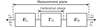
The artifacts introduced by a two-port measurement can be viewed as two linear circuits (left error box, right error box) cascaded in series with the DUT. All three circuits are represented as three matrices, called their S-parameters. Measurement error can be reduced by making error boxes nearly transparent using optimized port transitions. Alternatively, by mathematically removing the port’s contributions from the measured response using linear algebra, a process known as calibration or de-embedding (image by Ziad Hatab et al., licensed under CC BY-SA 4.0)
Implementation
Ports are a high-level concept in openEMS. Internally, they’re
implemented by first calling AddExcitation()
to create a source of EM field. Later, AddLumpedElement()
and AddProbe() are used to add termination
resistances and probes. One can create new port types based on these
low-level primitives.
Post-Processing
After the simulation is complete, a circuit’s frequency response or time-domain waveform is extracted to obtain meaningful results.
Attributes
Matlab / Octave |
Python |
Domain |
Definition |
|
|
Impedance |
Reference Impedance |
|
|
Frequency |
Incident Voltage |
|
|
Frequency |
Reflected Voltage |
|
|
Frequency |
Total Voltage |
|
|
Frequency |
Incident Current |
|
|
Frequency |
Reflected Current |
|
|
Frequency |
Total Current |
|
|
Frequency |
Incident Power |
|
|
Frequency |
Reflected Power |
|
|
Frequency |
Accepted Power (Incident - Reflected) |
N/A (see notes) |
|
Time |
Incident Voltage |
N/A (see notes) |
|
Time |
Reflected Voltage |
|
|
Time |
Total Voltage |
N/A (see notes) |
|
Time |
Incident Current |
N/A (see notes) |
|
Time |
Reflected Current |
|
|
Time |
Total Current |
|
|
Time |
Raw Voltage ( |
|
|
Time |
Raw Time of Voltage Samples |
|
|
Time |
Raw Current ( |
|
|
Time |
Raw Time of Current Samples |
Note
Voltage symbol. u is the unambiguous symbol of voltage (\(U\)) in ISO/IEC
convention,
so frequency-domain variables have the prefix uf, time-domain variables have the
prefix ut. In American literature, symbols such as \(V\), \(E\) and
\(\mathcal{E}\) are used.
Incident and reflected signals. In Matlab/Octave, only total time-domain port voltage and current are given, while their incident, reflected components are not. They can be calculated using the following expressions:
ut_inc = 0.5 * (ut_tot + it_tot * ZL_ref)
ut_ref = ut_tot - ut_inc

it_inc = 0.5 * (it_tot + ut_tot ./ ZL_ref)
it_ref = it_inc - it_tot
Usage
Matlab/Octave:
f_min = 100e6
f_max = 1e9
points = 1000
freq_list = linspace(f_min, f_max, points);

for i = 1:numel(port)
    port{i} = calcPort(port{i}, simpath, freq_list);
endfor

s11_list = port{1}.uf.ref ./ port{1}.uf.inc;
s21_list = port{2}.uf.ref ./ port{1}.uf.inc;
z21_list = port{1}.uf.tot ./ port{1}.if_tot;
Python:
import numpy as np
from matplotlib import pyplot as plt

f_min = 100e6
f_max = 1e9
points = 1000
z0 = 50
freq_list = np.linspace(f_min, f_max, points)

# after running the simulation
for p in port:
    p.CalcPort(simdir, freq_list, ref_impedance=z0)

s11_list = port[0].uf_ref / port[0].uf_inc
s21_list = port[1].uf_ref / port[0].uf_inc
z11_list = port[0].uf_tot / port[0].if_tot

plt.figure()
plt.plot(port[0].u_data.ui_time[0], port[0].ut_tot, label="Input Voltage")
plt.plot(port[1].u_data.ui_time[0], port[1].ut_tot, label="Output Voltage")
plt.grid()
plt.legend()
plt.xlabel('Time (s)')
plt.ylabel('Voltage (V)')
plt.show()
See also
Microstrip Notch Filter — lumped port setup on a microstrip structure.
Rectangular Waveguide — waveguide port with mode profile excitation.