Dipole Antenna Exposure & SAR
A half-wave dipole radiating next to a layered head phantom (skin, headbone, brain), used to calculate the Specific Absorption Rate (SAR) and the antenna’s power budget.
Introduction
This tutorial covers:
Setup of a layered ellipsoidal head phantom (skin, headbone, brain)
Disabling cell-averaging (
CellConstantMaterial) as required for SAR averaging per IEC/IEEE 62704-1Recording a SAR field dump and computing the 10g-averaged SAR
Calculating the antenna’s power budget: accepted, radiated (via NF2FF) and absorbed power
Python Script
Get the latest version from git.
Import Libraries
import os, tempfile
from matplotlib import pylab as plt
import numpy as np

from CSXCAD  import ContinuousStructure
from openEMS import openEMS
from openEMS.physical_constants import *
General parameter setup
Sim_Path = os.path.join(tempfile.gettempdir(), 'SAR_Dipole')
print(f'{Sim_Path=}')

# switches & options...
post_proc_only = False

# setup the simulation
unit = 1e-3 # all lengths in mm

f0 = 1e9 # center frequency
lambda0 = C0/f0

f_stop = 1.5e9 # 20 dB corner frequency
lambda_min = C0/f_stop

mesh_res_air = lambda_min/20/unit
mesh_res_phantom = 2.5

feed_R = 50 # feed resistance

# dummy phantom class to attach named attributes
class phantom:
    pass

# define phantom
phantoms = []
skin = phantom()
phantoms.append(skin)
skin.name='skin'
skin.epsR = 50
skin.kappa = 0.65 # S/m
skin.density = 1100 #  kg/m^3
skin.radius = [80, 100, 100] #  ellipsoide
skin.center = [100, 0, 0]

headbone = phantom()
phantoms.append(headbone)
headbone.name='headbone'
headbone.epsR = 13
headbone.kappa = 0.1 #  S/m
headbone.density = 2000 # kg/m^3
headbone.radius = [75, 95, 95] # ellipsoide
headbone.center = [100, 0, 0]

brain = phantom()
phantoms.append(brain)
brain.name='brain'
brain.epsR = 60
brain.kappa = 0.7 # S/m
brain.density = 1040 # kg/m^3
brain.radius = [65, 85, 85] # ellipsoide
brain.center = [100, 0, 0]
FDTD setup
Limit the simulation to 30k timesteps
Define a reduced end criteria of -40dB
Disabled advanced material cell interpolation and make sure to use an unaveraged constant cell material
This is less accurate but is required for SAR averaging according to IEC/IEEE 62704-1
FDTD = openEMS(NrTS=30000, EndCriteria=1e-4, CellConstantMaterial=True)
FDTD.SetGaussExcite( 0, f_stop )
FDTD.SetBoundaryCond( ['PML_8']*6 )

CSX = ContinuousStructure()
FDTD.SetCSX(CSX)
mesh = CSX.GetGrid()
mesh.SetDeltaUnit(1e-3)

dipole_length = 0.48*lambda0/unit
print(f'Lambda-half dipole length: {dipole_length:.1f} mm')

# Dipole
dipole = CSX.AddMetal('Dipole') # create a perfect electric conductor (PEC)
dipole.AddBox([0, 0, -dipole_length/2], [0, 0, dipole_length/2], priority=1)

# mesh lines for the dipole
thirds = np.array([-1/3, 2/3])
mesh.AddLine('z', -dipole_length/2-thirds*mesh_res_phantom)
mesh.AddLine('z', dipole_length/2+thirds*mesh_res_phantom)

# add the dielectrics
for n, ph in enumerate(phantoms):
    ph_mat = CSX.AddMaterial(ph.name, epsilon=ph.epsR, kappa=ph.kappa, density=ph.density)
    sp = ph_mat.AddSphere(priority=10+n, center=[0,0,0], radius=1)  #create a unit sphere, will be scaled and translated below
    tr = sp.GetTransform()
    tr.AddTransform('Scale', ph.radius)
    tr.AddTransform('Translate', ph.center)
    for dn, d in enumerate('xyz'):
        mesh.AddLine(d, [-1*ph.radius[dn]+ph.center[dn], ph.radius[dn]+ph.center[dn]])

# apply the excitation & resist as a current source
mesh.AddLine('x', [0])
mesh.AddLine('y', [0])
port = FDTD.AddLumpedPort(port_nr=1, R=feed_R, start=[-0.1, -0.1, -mesh_res_phantom/2], stop=[0.1, 0.1, +mesh_res_phantom/2], p_dir='z', excite=True)

mesh.SmoothMeshLines('all', mesh_res_phantom, 1.4)

# add lines for the air-box
mesh.AddLine('x', [-200, 350])
mesh.AddLine('y', [-250, 250])
mesh.AddLine('z', [-250, 250])
mesh.SmoothMeshLines('all', mesh_res_air, 1.4)

# dump SAR
start = [-30, -120, -120]
stop  = [200,  120,  120]
sar_dump = CSX.AddDump('SAR', dump_type=29, frequency=[f0], file_type=1, dump_mode=2)
sar_dump.AddBox(start, stop)

# nf2ff calc for power budget calculation
nf2ff = FDTD.CreateNF2FFBox()
Run the simulation
if 1 and not post_proc_only:  # debugging only
    CSX_file = os.path.join(Sim_Path, 'sar_dipole.xml')
    if not os.path.exists(Sim_Path):
        os.mkdir(Sim_Path)
    CSX.Write2XML(CSX_file)
    from CSXCAD import AppCSXCAD_BIN
    os.system(AppCSXCAD_BIN + ' "{}"'.format(CSX_file))

if not post_proc_only:
    FDTD.Run(Sim_Path, cleanup=True)
Post-processing and plotting
f = np.linspace(500e6, 1500e6, 501)
port.CalcPort(Sim_Path, f)
s11 = port.uf_ref/port.uf_inc
s11_dB = 20.0*np.log10(np.abs(s11))
plt.figure()
plt.plot(f/1e9, s11_dB, 'k-', linewidth=2, label='$S_{11}$')
plt.grid()
plt.legend()
plt.ylabel('S-Parameter (dB)')
plt.xlabel('Frequency (GHz)')
plt.title('S-Parameter')

Zin = port.uf_tot/port.if_tot

Pin_f0 = np.interp(f0, f, port.P_acc)

# plot feed point impedance
Zin = port.uf_tot/port.if_tot
plt.figure()
plt.plot(f/1e9, np.real(Zin), 'k-', linewidth=2, label=r'$\Re\{Z_{in}\}$')
plt.plot(f/1e9, np.imag(Zin), 'r--', linewidth=2, label=r'$\Im\{Z_{in}\}$')
plt.grid()
plt.legend()
plt.ylabel('Zin (Ohm)')
plt.xlabel('Frequency (GHz)')
plt.title('Input Impedance')


SAR_src = os.path.join(Sim_Path, 'SAR.h5') # calculated SAR output
SAR_fn = os.path.join(Sim_Path, 'SAR_10g.h5') # calculated SAR output
from openEMS.sar_calculation import  SAR_Calculation
if not os.path.exists(SAR_fn) or not post_proc_only:
    print('Calculate SAR')
    sar_calc = SAR_Calculation(mass=10, method='IEEE_62704')
    assert sar_calc.CalcFromHDF5(SAR_src, SAR_fn), 'SAR calculation failed'

from openEMS.sar_utils import readSAR

sar, mesh, sar_data = readSAR(SAR_fn)

max_sar = np.max(sar)

ptotal = float(sar_data['power'])
mass = float(sar_data['mass'])

theta = np.arange(0.0, 180.0, 5.0)
phi   = np.arange(0.0, 360.0, 5.0)
# The nf2ff far-field is calculated to determine the radiated power (that was not absorbed)
nf2ff_res = nf2ff.CalcNF2FF(Sim_Path, f0, theta, phi, center=[0,0,0], read_cached=post_proc_only, verbose=1)

print(f'max SAR: {max_sar/Pin_f0:.4g} W/kg normalized to 1 W accepted power')
print(f'whole body SAR: {ptotal/Pin_f0/mass:.4g} W/kg normalized to 1 W accepted power')
print(f'accepted power: {Pin_f0:.4g} W (100 %)')
print(f'radiated power: {nf2ff_res.Prad[0]:.4g} W ({100*(nf2ff_res.Prad[0]) / Pin_f0:.1f}%)')
print(f'absorbed power: {ptotal:.4g} W ({100*(ptotal) / Pin_f0:.1f}%)')
print(f'power budget:   {100*(nf2ff_res.Prad[0] + ptotal) / Pin_f0:.1f} %')  # this ideally should be within 95 to 100%

#  plot SAR on a x/y and x/z-plane
fig, axs = plt.subplots(1,2, figsize=(12, 5))

X,Y = np.meshgrid(mesh[0], mesh[1], indexing='ij')
Nz = len(mesh[2])
sar_xy = sar[:,:,Nz//2]
im = axs[0].pcolormesh(X,Y,sar_xy/Pin_f0, vmax=max_sar/Pin_f0)
axs[0].axis('equal')
axs[0].set_title('xy-plane')
plt.colorbar(im)
m_idx = np.unravel_index(np.argmax(sar_xy), sar_xy.shape)

X,Z = np.meshgrid(mesh[0], mesh[2], indexing='ij')
Ny = len(mesh[1])
sar_xz = sar[:,Ny//2,:]
im = axs[1].pcolormesh(X,Z,sar_xz/Pin_f0, vmax=max_sar/Pin_f0)
axs[1].axis('equal')
axs[1].set_title('xz-plane')
plt.colorbar(im)
fig.suptitle('Specific Absorbtion Rate (SAR)')

plt.show()
Images
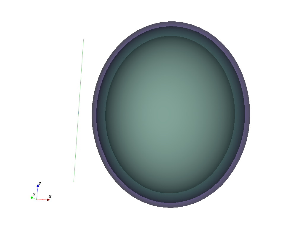
3D view of the half-wave dipole next to the layered head phantom (AppCSXCAD)
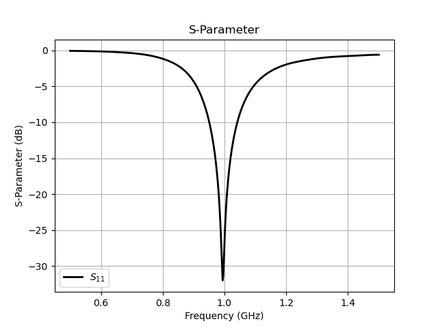
S-Parameter and input impedance of the dipole antenna
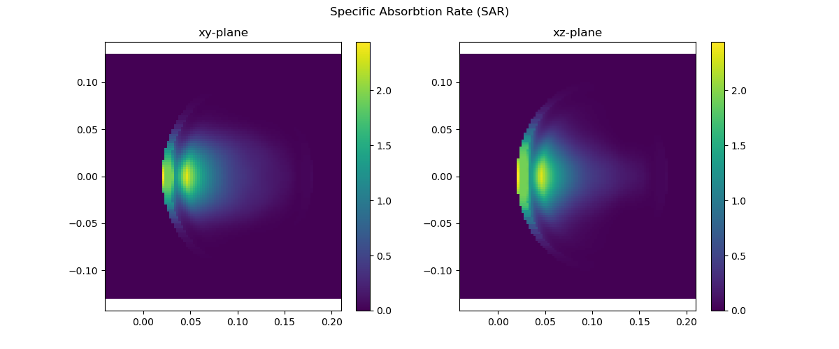
10g averaged SAR distribution on the xy- and xz-plane