Horn Antenna with Coaxial Pin Feed
A pyramidal horn antenna fed by a coaxial probe (pin) inside the rectangular feed waveguide, terminated by a quarter-wave back-short instead of a waveguide port.
Introduction
This tutorial covers:
Setup of a pyramidal horn antenna with a closed rectangular feed waveguide
A coaxial pin feed modelled as a lumped port, exciting the TE10 waveguide mode
A quarter guided-wavelength back-short instead of a waveguide port or PML termination
Calculate the S-Parameter and input impedance
Calculate the far-field pattern, directivity and aperture efficiency via NF2FF
Python Script
Get the latest version from git.
Import Libraries
import os, tempfile
import numpy as np
import matplotlib.pyplot as plt

from CSXCAD import ContinuousStructure
from openEMS import openEMS
from openEMS.physical_constants import *
Simulation path
Sim_Path = os.path.join(tempfile.gettempdir(), 'Horn_Antenna_PinFeed')

post_proc_only = False

unit = 1e-3     # all lengths in mm
Waveguide and Horn Parameters
a_wg = 20.0     # feed waveguide width  [mm] – TE10 propagates above fc = C0/(2a)
b_wg = 10.0     # feed waveguide height [mm]
wg_t  = 2.0     # metal wall thickness  [mm]

feed_length = 50.0  # length of the closed feed waveguide behind the horn mouth [mm]

horn_length = 50.0  # horn length in propagation direction (z) [mm]
horn_angle  = 20.0  # horn opening half-angle in both x and y [degrees]
Frequency
f_start = 10e9
f_stop  = 20e9
f0      = 15e9      # centre frequency of interest [Hz]
Derived parameters
fc_wg    = C0 / (2 * a_wg * unit)                          # TE10 cutoff [Hz]
lambda_g = C0/f0/unit / np.sqrt(1 - (fc_wg/f0)**2)        # guided wavelength at f0 [mm]

back_short = lambda_g / 4       # quarter-wave back-short [mm]
pin_length = b_wg * 0.55        # probe length [mm]  ← tune for best impedance match
pin_r      = 0.5                # probe cross-section half-width [mm] (≈ SMA inner conductor)
port_h     = 1.0                # lumped-port gap height at pin base [mm]
feed_R     = 50.0               # feed resistance [Ohm]

z_back = -feed_length           # inner face of the back-short wall [mm]
z_pin  = z_back + back_short    # pin position along the waveguide axis [mm]

# Horn aperture half-dimensions (at z = horn_length)
horn_ax = a_wg/2 + np.sin(np.deg2rad(horn_angle)) * horn_length
horn_ay = b_wg/2 + np.sin(np.deg2rad(horn_angle)) * horn_length

# Aperture area for antenna efficiency calculation
A_aperture = (2*horn_ax*unit) * (2*horn_ay*unit)

print(f'TE10 cutoff:            {fc_wg/1e9:.2f} GHz')
print(f'Guided wavelength at f0:{lambda_g:.2f} mm')
print(f'Back-short distance:    {back_short:.2f} mm')
print(f'Pin z-position:         {z_pin:.2f} mm  (from back wall: {back_short:.2f} mm)')
print(f'Pin length:             {pin_length:.2f} mm  (tune for matching)')
print(f'Pin cross-section:      {2*pin_r:.1f} x {2*pin_r:.1f} mm')
FDTD setup
FDTD = openEMS(EndCriteria=1e-4)
FDTD.SetGaussExcite(0.5*(f_start+f_stop), 0.5*(f_stop-f_start))
FDTD.SetBoundaryCond(['PML_8']*6)
Geometry and mesh
CSX = ContinuousStructure()
FDTD.SetCSX(CSX)
mesh = CSX.GetGrid()
mesh.SetDeltaUnit(unit)

max_res   = C0/f_stop/unit/20       # ≈ lambda/20 at highest frequency ≈ 0.75 mm

# Simulation box dimensions: structure edge + lambda/4 air gap + 8-cell PML estimate
lam0      = C0/f0/unit            # free-space wavelength at f0 [mm]
bc_offset = 9                     # PML_8 + 1 cell, matches CreateNF2FFBox placement
margin    = lam0/2 + bc_offset*max_res   # lambda/2 air gap + PML overhead [mm]

x_max     = horn_ax + margin      # x boundary (same margin used for y)
y_max     = horn_ay + margin      # y boundary
z_sim_back  = lam0/4 + bc_offset*max_res  # lambda/4 free space + PML overhead behind back wall
z_sim_front = margin              # in front of horn aperture: lambda/2 + PML

# Fixed mesh lines at key geometry locations
mesh.AddLine('x', [-x_max, -horn_ax, -(a_wg/2 + wg_t), -a_wg/2, -pin_r, pin_r,
                   a_wg/2, a_wg/2 + wg_t, horn_ax, x_max])
mesh.AddLine('y', [-y_max, -horn_ay, -(b_wg/2 + wg_t), -b_wg/2,
                   -b_wg/2+port_h, -b_wg/2+pin_length,
                   b_wg/2, b_wg/2 + wg_t, horn_ay, y_max])
mesh.AddLine('z', [z_back - z_sim_back, z_back - lam0/4, z_back - wg_t, z_back,
                   z_pin-pin_r, z_pin+pin_r,
                   0, horn_length, horn_length + z_sim_front])
Create horn antenna geometry
horn = CSX.AddMetal('horn')
Feed waveguide walls (closed rectangular tube from z_back to z=0)
# left wall  (at x = -a_wg/2)
horn.AddBox(priority=10, start=[-a_wg/2 - wg_t, -b_wg/2, z_back], stop=[-a_wg/2, b_wg/2, 0])
# right wall (at x = +a_wg/2)
horn.AddBox(priority=10, start=[ a_wg/2, -b_wg/2, z_back], stop=[ a_wg/2 + wg_t, b_wg/2, 0])
# top wall   (at y = +b_wg/2)
horn.AddBox(priority=10, start=[-a_wg/2 - wg_t,  b_wg/2,        z_back], stop=[ a_wg/2 + wg_t,  b_wg/2 + wg_t, 0])
# bottom wall (at y = -b_wg/2)
horn.AddBox(priority=10, start=[-a_wg/2 - wg_t, -b_wg/2 - wg_t, z_back], stop=[ a_wg/2 + wg_t, -b_wg/2,        0])
Back-short wall (metal lid closing the waveguide)
horn.AddBox(priority=10,
            start=[-a_wg/2 - wg_t, -b_wg/2 - wg_t, z_back - wg_t],
            stop= [ a_wg/2 + wg_t,  b_wg/2 + wg_t,  z_back       ])
Flared horn walls (four trapezoidal plates, one per side)
#
# LinPoly coordinate convention (from CSXCAD C++ cyclic index formula):
#   norm_dir='y': points[0] = z-coords, points[1] = x-coords
#   norm_dir='x': points[0] = y-coords, points[1] = z-coords
#
# Each plate starts in the plane of its normal direction at y/x = 0,
# is extruded by wg_t (centred on the elevation), then transformed with
# a rotation (to create the flare angle) and a translation (to the waveguide edge).

# Shared z-coordinates for the top/bottom horn-wall polygon
z_tb = np.array([0, horn_length, horn_length, 0])
# Corresponding x-coordinates (trapezoid widening along z)
x_tb = np.array([ a_wg/2, a_wg/2 + np.sin(np.deg2rad(horn_angle))*horn_length,
                 -a_wg/2 - np.sin(np.deg2rad(horn_angle))*horn_length, -a_wg/2])

# Bottom horn wall: rotate +horn_angle around x → far end tilts to −y
p = horn.AddLinPoly(points=[z_tb, x_tb], norm_dir='y',
                    elevation=-wg_t/2, length=wg_t, priority=10)
p.AddTransform('RotateAxis', 'x',  horn_angle)
p.AddTransform('Translate', [0, -b_wg/2 - wg_t/2, 0])

# Top horn wall: rotate −horn_angle around x → far end tilts to +y
p = horn.AddLinPoly(points=[z_tb, x_tb], norm_dir='y',
                    elevation=-wg_t/2, length=wg_t, priority=10)
p.AddTransform('RotateAxis', 'x', -horn_angle)
p.AddTransform('Translate', [0,  b_wg/2 + wg_t/2, 0])

# Shared y-coordinates for the left/right horn-wall polygon
# (spans full waveguide height including wall thickness, flares outward in y)
y_lr = np.array([ b_wg/2 + wg_t, b_wg/2 + wg_t + np.sin(np.deg2rad(horn_angle))*horn_length,
                 -b_wg/2 - wg_t - np.sin(np.deg2rad(horn_angle))*horn_length, -b_wg/2 - wg_t])
z_lr = np.array([0, horn_length, horn_length, 0])

# Left horn wall: rotate −horn_angle around y → far end tilts to −x
p = horn.AddLinPoly(points=[y_lr, z_lr], norm_dir='x',
                    elevation=-wg_t/2, length=wg_t, priority=10)
p.AddTransform('RotateAxis', 'y', -horn_angle)
p.AddTransform('Translate', [-a_wg/2 - wg_t/2, 0, 0])

# Right horn wall: rotate +horn_angle around y → far end tilts to +x
p = horn.AddLinPoly(points=[y_lr, z_lr], norm_dir='x',
                    elevation=-wg_t/2, length=wg_t, priority=10)
p.AddTransform('RotateAxis', 'y',  horn_angle)
p.AddTransform('Translate', [ a_wg/2 + wg_t/2, 0, 0])
Coaxial pin feed
# The feed is split into two parts that together model a coaxial probe:
#
#   ┌──────┐  ← pin tip      (y = −b_wg/2 + pin_length)
#   │ PEC  │  ← metal pin body (CSX metal box, cross-section 2*pin_r × 2*pin_r)
#   │ pin  │
#   └──────┘  ← port top     (y = −b_wg/2 + port_h)
#   [lumped]  ← short port gap modelling the coaxial connector transition
#  ══════════ ← bottom wall   (y = −b_wg/2)

# Short lumped port (the coaxial connector gap, same cross-section as pin body)
start = [-pin_r, -b_wg/2,          z_pin - pin_r]
stop  = [ pin_r, -b_wg/2 + port_h, z_pin + pin_r]
port = FDTD.AddLumpedPort(1, feed_R, start, stop, 'y', 1.0, priority=5)

# Metal pin body (PEC post from port top to pin tip, realistic cross-section)
pin_metal = CSX.AddMetal('pin')
pin_metal.AddBox(priority=10,
                 start=[-pin_r, -b_wg/2 + port_h,  z_pin - pin_r],
                 stop= [ pin_r, -b_wg/2 + pin_length, z_pin + pin_r])
Smooth mesh and create NF2FF recording box
mesh.SmoothMeshLines('all', max_res, 1.4)
nf2ff = FDTD.CreateNF2FFBox()
Optional: write XML and launch AppCSXCAD for geometry inspection
if 1:
    CSX_file = os.path.join(Sim_Path, 'horn_pinfeed.xml')
    if not os.path.exists(Sim_Path):
        os.mkdir(Sim_Path)
    CSX.Write2XML(CSX_file)
    from CSXCAD import AppCSXCAD_BIN
    os.system(AppCSXCAD_BIN + ' "{}"'.format(CSX_file))
Run the simulation
if not post_proc_only:
    FDTD.Run(Sim_Path, cleanup=True)
Post-processing
freq = np.linspace(f_start, f_stop, 401)
port.CalcPort(Sim_Path, freq)

s11    = port.uf_ref / port.uf_inc
s11_dB = 20.0 * np.log10(np.abs(s11))
Zin    = port.uf_tot / port.if_tot
Reflection coefficient S11
fig, ax = plt.subplots(num='S11', tight_layout=True)
ax.plot(freq/1e9, s11_dB, 'k-', linewidth=2)
ax.axhline(-10, color='gray', linestyle='--', linewidth=1)
ax.grid()
ax.set_xmargin(0)
ax.set_ylim([-40, 5])
ax.set_xlabel('Frequency (GHz)')
ax.set_ylabel('S11 (dB)')
ax.set_title('Reflection Coefficient S11')
Input impedance
fig, ax = plt.subplots(num='Zin', tight_layout=True)
ax.plot(freq/1e9, np.real(Zin), 'k-',  linewidth=2, label=r'$\Re\{Z_{in}\}$')
ax.plot(freq/1e9, np.imag(Zin), 'r--', linewidth=2, label=r'$\Im\{Z_{in}\}$')
ax.grid()
ax.set_xmargin(0)
ax.set_xlabel('Frequency (GHz)')
ax.set_ylabel('Impedance (Ohm)')
ax.set_title('Input Impedance')
ax.legend()
Far-field radiation pattern at f0
theta = np.arange(-180.0, 180.0, 2.0)
phi   = [0.0, 90.0]
print(f'Calculating far field at f0 = {f0/1e9:.1f} GHz ...')
nf2ff_res = nf2ff.CalcNF2FF(Sim_Path, f0, theta, phi)

Dmax_dBi = 10.0 * np.log10(nf2ff_res.Dmax[0])
G_a = 4 * np.pi * A_aperture / (C0/f0)**2      # ideal aperture gain (uniform illumination)
e_a = nf2ff_res.Dmax[0] / G_a                  # aperture efficiency

print(f'Directivity:          Dmax = {Dmax_dBi:.1f} dBi')
print(f'Aperture efficiency:  e_a  = {e_a*100:.1f} %')

E_norm = (20.0*np.log10(nf2ff_res.E_norm[0] / np.max(nf2ff_res.E_norm[0]))
          + Dmax_dBi)

fig, ax = plt.subplots(num='Pattern', tight_layout=True)
ax.plot(theta, E_norm[:, 0], 'k-',  linewidth=2, label='E-plane  (phi=0°)')
ax.plot(theta, E_norm[:, 1], 'r--', linewidth=2, label='H-plane  (phi=90°)')
ax.grid()
ax.set_xmargin(0)
ax.set_xlabel('Theta (deg)')
ax.set_ylabel('Directivity (dBi)')
ax.set_title(f'Far-Field Pattern at {f0/1e9:.1f} GHz')
ax.legend()

plt.show()
Images
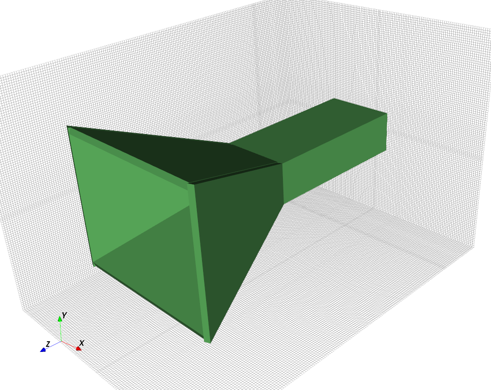
3D view of the Horn Antenna with coaxial pin feed (AppCSXCAD)
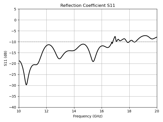
S-Parameter of the horn antenna
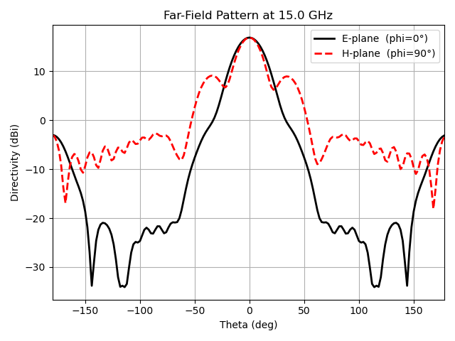
Farfield pattern on an E- and H-plane